Rarecoal
Histogram files
Rarecoal reads data in the form of a joint allele frequency histogram for rare alleles. An example file can be found under exampleData/fourPop.histogram.txt in the rarecoal repository. The first lines look like this:
NAMES=EUR,SEA,SIB,FAM
N=66,44,44,28
MAX_M=10
TOTAL_SITES=1146826657
1,0,0,0 1525898
0,1,0,0 1075097
0,0,1,0 818979
0,0,0,1 433157
2,0,0,0 315625
...
The first line denotes the names of the populations. These names are used when specifying models. Names can contain letters, numbers, underscores and hyphens. The second line denotes the number of haploid samples in each subpopulations. In this case there are four subpopulations, with 33, 22, 22 and 14 diploid individuals in the four populations, and twice the number of haplotypes. The third line denotes the maximum total allele count of variants, here 10, so up to an allele freuqency \(10/182\approx 5\%\). The fourth line denotes the total number of sites considered, which is important to use the mutation clock to time events and estimate branch effective population sizes.
The lines from line 5 are pairs of patterns and numbers separated by a space or a tab. A pattern describes how a mutation is distributed across the populations. In the example above, for a variant of allele frequency 5, there could be a pattern of the form 0,2,2,1, which means that there are zero derived mutations in the first, two in the second and third population, and one in the fourth population. The special pattern HIGHER summarizes all variants with total allele frequency higher than denoted by the MAX_M line in the file. The number after each pattern is the number of sites in the data set that exhibit this particular pattern.
Warning
Note that in previous versions of rarecoal, there were two special patterns, 0,0,0,0 (with as many zeros as populations) and HIGHER. This is not anymore valid.
I provide tools for generating this format from VCF and Eigenstrat files within the rarecoal-tools package, notably vcf2FreqSum, eigenstrat2FreqSum and freqSum2Histogram.
Tip
In all of my tools, you can get an online help using the option -h. This works in particular for rarecoal by typing rarecoal -h, and for a specific subcommand, say mcmc, by typing rarecoal mcmc -h.
Scaled Units
All time inputs and outputs in rarecoal are measured in units of \(2N_0\) generations, and all population sizes are measured in units of \(N_0\). Here, \(N_0\) is indirectly set using the --theta option in any rarecoal command, which is a constant defined as \(2N_0\mu\), where \(\mu\) is the per-generation mutation rate. By default, theta is set to 0.0005, which for humans corresponds to \(N_0=20,000\) assuming a per-generation mutation rate of \(\mu=1.25\times 10^{-8}\).
Note
I apologize to all Population Geneticists for using a factor 2 instead of 4 in the definition of theta.
In order to convert scaled population size estimates to real population sizes, multiply by \(N_0\), and in order to convert scaled time to the number of generations, multiply by \(2N_0\). To convert generations to years, multiply by the generation time (e.g. 29 years for humans).
Multithreading
Rarecoal by default runs in parallel on as many cores as it can find on your machine. If you want to specify the number of threads explicitly, for example in order to restrict the number of cores, you can do that using the --nrThreads option. In my experience, the speed increases fairly linearly up to around 8 processors. Up to around 16 processors, there is still some improvement, but much slower than linear. So I would usually recommend running on 8 processors at most, although you can try to go higher if you can afford it.
Demographic models
For many rarecoal subcommands, a demographic model needs to be specified. This can be done either through a model file (as in exampleData/fourPop.template.txt), passed via option -T <FILE> or via the command line using option -t <STRING>. When using the second option, you can skip the newlines shown in the following example. In both cases, the model specification has the same syntax. Here is the example from exampleData/fourPop.template.txt:
BRANCHES = [EUR, SEA, SIB, FAM]
EVENTS = [
        P 0.0 EUR <p_EUR>;
        P 0.0 SEA <p_SEA>;
        P 0.0 SIB <p_SIB>;
        P 0.0 FAM <p_FAM>;
        K <t_EUR_SIB>    EUR SIB <p_EUR_SIB>;
        K <t_SEA_FAM>    SEA FAM <p_SEA_FAM>;
        K <t_EUR_SEA>    EUR SEA <p_EUR_SEA>;
        S <tAdm_FAM_SIB> FAM SIB <adm_FAM_SIB>;
        P <tAdm_FAM_SIB> FAM     <pAdm_FAM_SIB>;
        S <tAdm_SEA_SIB> SEA SIB <adm_SEA_SIB>;
        P <tAdm_SEA_SIB> SEA     <pAdm_SEA_SIB>;
        S 0.00022        EUR FAM <adm_EUR_FAM>
]
CONSTRAINTS = [
        C <tAdm_FAM_SIB> > 0.00022
]
The first expression specifies the branches used in the model, here there are four, named EUR, SEA, SIB, FAM. The second expression specifies the demographic events, separated by semicolons, which are by convention ordered going backwards in time. This is very similar to simulation software like ms or msPrime.
Note
Note that the semicolon is used only for separating events, so the last event should not end with a semicolon. Newlines are always optional, as well as white spaces after closed squared brackets and semicolons.
As an example input of a (less complex) model via the command line, consider -t "BRANCHES = [EUR, SEA, SIB] EVENTS = [J <t_SEA_SIB> SEA SIB; J <t_EUR_SEA> EUR SEA]. At the moment, rarecoal supports the following type of events:
- Population Size Changes
- These are specified using an expression of the sort
P <time> <branch> <size>, and change the population size on branch<branch>at time<time>to new size<size>(see ScaledUnits for how to scale population sizes and times). By default, all branch population sizes are set to \(1\) in scaled units, i.e. \(N_0\) in real units. In a forward-in-time perspective, these events affect the population size in a branch prior to the specified time. - Join Events
- These are specified using an expression of the sort
J <time> <branch_k> <branch_l>, and move all lineages from<branch_l>into branch<branch_k>. In a forward-in-time perspective, these events are denote population splits, where the new<branch_l>splits off from the<branch_k>. - Split events
- Split events are specified using an expression of the sort
S <time> <branch_k> <branch_l> <fraction>, which moves lineages with rate<fraction>from<branch_l>to branch<branch_k>. In a forward-in-time perspective these events are admixture events from<branch_k>into<branch_l>. - Join-Popsize Events
- When we model a population join, we often want to allow the ancestral branch to have a separate population size. Rarecoal therefore provides a combined event type for convenience, specified using an expression of the form
K <time> <branch_k> <branch_l> <size>, which specifies that at time<time>, all lineages from<branch_l>are to be moved into<branch_k>, and a subequent population size change in<branch_k>to the new population size<size>. - Freeze Events
- This is a special event, used for modelling ancient samples/populations. A freeze event is specified via
F <time> <branch> TrueorF <time> <branch> False. See BranchShortening below.
Ghost Branches
Any branch that occurs in the model template, but not in the histogram file is called a ghost branch. Such a branch is unsampled (no ancient or modern population listed in the histogram file corresponds to it), but lineages can be moved into it and out of it using standard demographic events such as Join and Split.
Free Parameters
As you can see in the example above, instead of providing concrete values for event times, population sizes and admixture rates, you can provide a named parameter, specified using a syntax of the form <parameter_name>, enclosed by symbols < and >. These free parameters need to be set or initialised either via a parameter file (see below), or via the command line using the option -X name=value as many times as needed to specify all parameters.
Tip
Option -X can also be used on top of providing a parameter file, which then overwrites the parameter read from the file in that case.
As an example, consider this simple use of rarecoal prob (see below):
rarecoal prob -t "BRANCHES=[P1,P2] EVENTS=[J <t_P1_P2> P1 P2]" -X t_P1_P2=0.01 [100,100] [1,1]
This command would fail without the option -X t_P1_P2=0.01, since the model would have a free parameter that is not specified.
Parameter Files
A convenient way to input values for free parameters are parameter files, using the option -P <FILE>. The simplest form is a file like this:
param1 1.5
param2 3.6
...
which simply lists all parameters with their values row by row. Conveniently, this format is exactly the format output by rarecoal maxl, which makes it easy to run a model using previous parameter estimates (for example from a simpler model) as input, and then using the command line option -X to specify the parameters not listed in that file.
As another convenience, rarecoal also tolerates reading in the output parameter estimation files from rarecoal mcmc, which also contains confidence intervals that are however ignored here. Rarecoal detects automatically, whether an input parameter file has the simple rarecoal maxl format described above, or the more complicated rarecoal mcmc format. In any case, you can use these output files as parameter input files using the -P option.
Constraints
While the BRANCHES and EVENTS expressions are mandatory in specifying a model, the CONSTRAINTS expression is optional. When used, it should contain expressions of the sort C <parameter1> > <parameter2> or C <parameter1> < <parameter2>, again separated by semicolons. Here, <parameter1> is always a named parameter surrounded by < and >, while <parameter2> can either be a named parameter or a number, as in the example above. Constraints are important for parameter inference (see maxl and mcmc commands), in which case the inference is guaranteed to satisfy the constraints. If initial parameters violate the constraints, an error is thrown.
Excluding singletons and private variants
Low coverage samples, in particular ancient samples, often have a higher false-positive rate for derived variants than modern high coverage samples. False positive derived variants are typically seen as private singletons in the ancient sample. This can severely affect estimates of branch lengths leading to ancient samples. Rarecoal therefore allows to exclude singletons and private variants from computing the likelihood of the data given a model. This can be specified using the --excludePattern flag, which can be generally used to exclude particular mutational patterns from computing the likelihood, or from fitting.
Example: --excludePattern [0,0,0,1,0] --excludePattern [0,0,0,2,0] would specify that any singletons and private doubletons in the fourth population would be excluded from the likelihood calculation (and hence from model fits).
Branch Shortening
In order to model an ancient individual at its correct sampling time, you an specify the age of a sample using a model feature called branch freezing. Consider an ancient sample that died a specific time ago, say 0.05 in scaled units. The model should then specify that between now (time 0) and time 0.05 in the past there should not be any coalescence events within that branch. You can freeze or unfreeze specific branches with a particular demographic “freeze event”. Freeze events are specified using the F <time> <branch> True/False. Events with True freeze branch <branch> at time <time>. Events with False unfreeze that branch.
Example: F 0.0 AncientSample True; F 0.05 AncientSample False. Here we specify that an ancient sample in a branch named “AncientSample” died at time 0.05.
Computing the probability of a particular mutation pattern (rarecoal prob)
This is a basic command that lets you compute the probability for a particular mutation pattern using rarecoal. As an example, try:
rarecoal prob -t "BRANCHES=[P1,P2] EVENTS=[J 0.02 P1 P2]" [100,100] [1,1]
which computes the probability to observe a shared doubleton in two populations that split at time 0.02 in the past, each with 100 sampled haplotypes. Here, the two arguments [100,100] and [1,1] specify that each population contains 100 haplotypes, and we are computing the frequency of the pattern [1,1], i.e. a doubleton shared by both populations. The output of this command is:
Rarecoal starting at 2018-07-12 10:46:17.93554 UTC
running on 4 processors
loaded model template with branch names ["P1","P2"], events [MTJoin (ParamFixed 2.0e-2) "P1" "P2"], constraints [] and parameters []
6.134185013046277e-5
Rarecoal finished at 2018-07-12 10:46:17.950171 UTC
where the first three and the last line are log outputs, printed to standard error, and the second line contains the result, printed to standard out.
Tip
You can make the log outputs disappear by piping the error output into nothing, via rarecoal CMD OPTS 2> /dev/null.
I have included this program mainly for debugging purposes, to test model templates, and to investigate the numerical accuracy of the underlying approximations (compared to exact analytical calculations or full coalescent simulations).
A more complex example involving a template would be:
rarecoal prob -T exampleData/fourPop.template.txt \
-P exampleData/fourPop.m4.mcmc.paramEstimates.txt -X p_EUR=2 \
[100,100,100,100] [1,1,2,1] 2> /dev/null
where I am using the files in the exampleData directory in the rarecoal repository. Note that in this example, I used the feature of using the -X option to overwrite a parameter read from the parameter input file. The result of this computation is:
3.0848062621032846e-7
which is the probability to observe a variant of allele count 5 shared by all four populations (two alleles in branch SIB and 1 in all other populations) under the model specified by the template exampleData/fourPop.template.txt and the parameter file exampleData/fourPop.m4.mcmc.txt. Here, the parameter file contains numerical estimates for all parameters, as returned by rarecoal mcmc, as covered further below.
Tip
Type rarecoal prob -h to get a list of all command line options.
Note
Modelling Ghost branches in rarecoal prob requires you to set the number of haplotypes in that branch explicitly to zero. This is different from commands that use a histogram, in which all model branches that do not occur in the histogram file are by definition ghost branches.
Computing the likelihood of a histogram data set given a model (rarecoal logl)
While rarecoal prob allows us to compute the probability for a particular mutational pattern under a model, rarecoal logl lets us use these probabilities to compute the likelihood of an entire allele frequency spectrum given a model.
The command takes a model (specified either via the command line or via a template) and a Histogram file, and spits out the log likelihood for the histogram under that particular model. Here is an example, again using the data in the exampleData folder in the rarecoal repository:
rarecoal logl -T exampleData/fourPop.template.txt \
-P exampleData/fourPop.m4.mcmc.paramEstimates.txt -m2 \
-i exampleData/fourPop.histogram.txt 2> /dev/null
Here, the flag -m2 specifies that the computation should include only variants up to allele count 2, so singletons and doubletons. The command outputs:
-4.3434710950368606e7
which gives the log-likelihood of the data given the model.
Tip
Type rarecoal logl -h to get a list of all command line options.
Parameter estimation using likelihood maximization (rarecoal maxl)
This command instructs rarecoal to perform a numerical optimization of the parameters of a model given the data. For this command, you must provide a model via a template (see above).
A usage example using the example data is:
rarecoal maxl -T exampleData/fourPop.template.txt --nrThreads 8 -o out \
-i exampleData/fourPop.histogram.txt -P exampleData/fourPop.m4.mcmc.paramEstimates.txt --powell
This will take around five minutes on 8 cores. Note that here I initialised the run using a parameter file. If a parameter is not given in the file, and not set via option -X through the command line, rarecoal will try to guess what how it should be initialised: If it is a parameter starting with p, it will assume that the parameter specifies a population size and initialise it with 1 (scaled units). If it starts with adm, it assumes that the parameter specifies an admixture rate and initialise it with 0.05. If it starts with t or any other letter, it will throw an error and demand an explicit initial value.
Tip
Always use the --powell flag when running rarecoal maxl. It’s the by far superior optimization method, compared to the default, which is the Nelder-Mead-Simplex method. I will in the future declare Powell’s method as default, but for now you need to use this flag to indicate that you want to use it.
Tip
Type rarecoal maxl -h for other command line options.
This command will output four files, all starting with the prefix entered via -o. The four files are:
<PREFIX>.paramEstimates.txt- a file containing the maximum likelihood parameter estimates<PREFIX>.frequencyFitTable.txt- a file containing the observed and expected frequency of each mutational pattern<PREFIX>.summaryFitTable.txt- a file containing the observed and expected average allele sharing summary statistics for private and shared vairants.<PREFIX>.trace.txt- A file containing the optimization path for all parameters.
Most of these files should be self-explanatory, but we highlight one very useful diagnostic file which may be less trivial: The *.summaryFitTable.txt file looks like this:
Populations AlleleSharing   Predicted       relDev%
EUR(singletons)     7.029790255707617e-4    7.036112569435226e-4    0
SEA(singletons)     4.952956498101769e-4    4.920355535110557e-4    -1
SIB(singletons)     3.773024536259415e-4    3.6244510637277715e-4   -4
FAM(singletons)     1.9955481020301124e-4   2.0312245044686625e-4   2
EUR/EUR     3.1980148283336265e-7   3.247373451950278e-7    2
EUR/SEA     3.8530518501698e-8      4.8016859495293024e-8   25
EUR/SIB     1.0808458019464607e-7   1.0200396524745371e-7   -6
EUR/FAM     4.1320772656606e-8      4.154205656954864e-8    1
SEA/SEA     2.709608862543286e-7    3.1390805761148254e-7   16
SEA/SIB     1.0389823577411024e-7   9.738061985956165e-8    -6
SEA/FAM     3.4037472303368755e-8   4.403202216655752e-8    29
SIB/SIB     4.2373651859060487e-7   3.063120490646186e-7    -28
SIB/FAM     8.378244737090708e-8    6.443081353680432e-8    -23
FAM/FAM     3.226852220082246e-7    3.729786700694564e-7    16
This file gives for each type of pattern the observed and predicted allele sharing, as well as a relative deviation between the two in percent. Rare allele sharing is essentially the rate of matching derived rare alleles between two haploid genomes. “Rare” here means whatever allele count cutoff was used in the run (by default, up to allele count of 4 in the entire sample set). The patterns with “(singletons)” are special and simply denote the rate of singletons per haploid genome.
As you can see in this case, all deviations are smaller than 30%, which is not too bad a fit. One feature to look for in this file are patterns with clear underestimations of allele sharing between two different populations between model and data. In this example, consider the SIB/FAM sharing (which denotes rare allele sharing between Siberians and Native Americans, by the way). which the model underestimates with 23%. This would be a candidate to introduce an admixture edge between the two populations to bring up their allele sharing.
Note
In all likelihood-based commands, in particular in maxl and mcmc, population size changes are subject to regularization penalties, which tries to avoid too drastic changes in population sizes. The strength of this effect can be controlled using the --regularization flag, which is available in most commands. By default, this value is 10.0 and to switch off, set it to zero.
Parameter estimation using Markov Chain Monte Carlo (rarecoal mcmc)
Parameter estimation using MCMC works very similarly as for the maxl command. The example from above will work just like before, but with a different command:
rarecoal mcmc -T exampleData/fourPop.template.txt --nrThreads 8 -o out \
-i exampleData/fourPop.histogram.txt -P exampleData/fourPop.m4.mcmc.paramEstimates.txt
This takes longer than rarecoal maxl, but gives more confidence that the result is actually a true local optimum. In addition, it gives confidence intervals for each parameter (however, see Effective Nr of sites correction for MCMC). The four files are exactly the same as for rarecoal maxl. Here is the resulting *.paramEstimates.txt file:
# Nr Burnin Cycles: 1346
# Nr Main Cycles: 1001
Param       MaxL    LowerCI Median  UpperCI
Score       5.503134217048233e7     5.503134452615323e7     5.5031350645868205e7    5.503135954187898e7
p_EUR       1.9060110218875406      1.895296943665767       1.910033905348887       1.9235488250218107
p_SEA       6.67308272111562        6.574244580495408       6.654234276295017       6.756639725275574
p_SIB       0.7322555089809326      0.7291216777996752      0.7326601729756712      0.7366083653316352
p_FAM       1.2005608490867878      1.180947811365368       1.1969363365988537      1.2041826385414909
t_EUR_SIB   1.5951118620536157e-2   1.582233044091577e-2    1.5939419201797773e-2   1.6071751484740902e-2
t_SEA_FAM   2.3579877111286916e-2   2.349314643161468e-2    2.3589085078451866e-2   2.3652342753859978e-2
t_EUR_SEA   2.682133249619095e-2    2.6733648526926033e-2   2.6819764941774262e-2   2.6908951869738077e-2
p_EUR_SIB   0.6758664106500165      0.6630959460319203      0.6739730521293578      0.6843019660858418
p_SEA_FAM   0.1178131584592131      0.11636887405941267     0.11807528006682372     0.12463816645062352
p_EUR_SEA   0.703514679898969       0.7011523891765922      0.7032195341665299      0.705588895959717
tAdm_FAM_SIB        9.266895562735303e-3    9.216772787832948e-3    9.307353281282293e-3    9.39751360656597e-3
pAdm_FAM_SIB        0.1200782357355394      0.11816164996954927     0.11977846738938136     0.12048497575822906
adm_FAM_SIB 0.14724562235805613     0.14596805017223682     0.14752533165513468     0.1490757530856995
adm_EUR_FAM 8.224165635046557e-2    8.121552240657676e-2    8.217924116309754e-2    8.315994460052621e-2
tAdm_SEA_SIB        1.1353430075486814e-2   1.1195086830652012e-2   1.133154960560658e-2    1.143206296087407e-2
pAdm_SEA_SIB        0.6674934743296429      0.6603972140580212      0.6674210400205404      0.6776177061340379
adm_SEA_SIB 0.3731833140538629      0.3699711973205964      0.37335715822805615     0.3757981722172729
The first two lines contain the number of burnin cycles and main MCMC cycles performed. The third line is a header row. All other rows contain Maximum likelihood estimates for each parameter, as well as the Median and upper and lower 95% confidence interval boundary for each parameter. The trace file in this case also contains more information than with rarecoal maxl, now giving also the adapted proposal width, as well as the proposal success rate for each parameter and each cycle.
Note
Each MCMC cycle consists of a proposal for each parameter in turn. Proposal width are adapted regularly to keep the acceptance rate around 50%. The run is stopped when the likelihood did not substantially change within 1000 cycles. So the number of non-burnin cycles is by definition 1000 (actually 1001). You can change the required number of main cycles using the --cycles flag.
Tip
Type rarecoal mcmc -h for other command line options.
Adding a branch to a model (rarecoal find)
Rarecoal find performs a brute force search for the branch point of a subpopulation branch, given a partial model. There are two use cases for this program. First, you can use rarecoal find to iteratively find the optimal model topology for a number of populations. For example, let’s say I already know how the first four populations in a five-population model are related, and let’s say their so-far best four-population model is given by a series of joins, specified on the command line by -t “BRANCHES=[P1,P2,P3,P4,P5] EVENTS=[J 0.0025 P1 P2; J 0.005 P3 P4; J 0.01 P1 P3]”. We can then use rarecoal find to find the maximum likelihood merge-point for the fifth population onto that model, via:
rarecoal find -t "BRANCHES=[P1,P2,P3,P4,P5] EVENTS=[J 0.0025 P1 P2; J 0.005 P3 P4; J 0.01 P1 P3]" -q 4 -f out_eval.txt -n P5 -i <Some.5pop.histogram>
Here, the parameter -n P5 specifies that we are trying to find the merge-point of branch P5, -f gives the file where to write the likelihood of each tried point to. Here, <5pop.histogram> should be replaced by the histogram file for the full data set including the population that you are trying the merge point for.
The second use case is for placing individual samples onto a tree. Let’s say you have optimized a full model including population sizes in each branch for your five populations, with the final MCMC output stored in mcmc_out.txt. You have generated a new histogram for these five populations plus one individual of unknown ancestry. Let’s say your individual is an ancient sample, with a sampling age 2,000 years before present. Scaling with \(2N<sub>0</sub>=20,000\) (see scaling note above), and a generation time of 29 years, the scaled age is then 0.00172. Then for mapping the individual, you would run:
rarecoal find -T <TEMPLATE> -P mcmc_out.txt -m 4 -n AncientSample -f mapping_out.txt -b 0.00172 -i <5pop.histogram>
Notice that we here used the optional parameter -b to set a scaled sampling age. The standard output of the rarecoal find command is simply the maximum likelihood branch point, specified via a branch index (0-based) and a time. The index refers to the branches specified in the template, not the histogram! The evaluation file specified using -f contains as additional information all likelihoods at all tried branch positions.
Tip
Type rarecoal find -h for other command line options.
Investigating model fits (rarecoal fitTable)
This program takes as input a histogram, a template specification and parameter specifications. It then prints a table with real and fitted probabilites for singletons and shared variants up to an allele count specified on the command line. For example:
rarecoal fitTable -T exampleData/fourPop.template.txt -P exampleData/fourPop.m4.mcmc.paramEstimates.txt -i exampleData/fourPop.histogram.txt -o out
The resulting tables are again written to files using the prefix specified using -o and are of the same format as the corresponding *.summaryFitTable.txt and *.frequencyFitTable.txt files output from rarecoal maxl and rarecoal mcmc.
Tip
Type rarecoal fitTable -h for other command line options.
Simulating a model (rarecoal simCommand)
This is a useful little command that outputs a model in the format as used in simulation software such as ms and msPrime.
Tip
Type rarecoal simCommand -h for other command line options.
Effective Nr of Sites correction
This is a new feature that is critical to obtain reasonable confidence intervals for your parameter. Support and documentation is still a bit rough, and I will try to automate the process in the future.
Rarecoal uses a composite likelihood approach, which simply computes the total likelihood of the data given a model as the product of probabilities across all sites. This approach neglects linkage among sites, which does not affect the maximum likelihood parameter estimates. However, composite likelihoods can not be used to compute posterior distributions or asses significance of model comparisons.
We can solve this issue by correcting the composite likelihood by a factor that reflects the effective number of independent sites, which is much smaller than the true number of sites analyzed. To estimate the reduction factor of the likelihood, we first use a simple Block-Jackknife procedure to estimate the sampling variance of the joint allele frequency spectrum (Busing et al. 1999). Jackknife error estimation is built into the program freqSum2Histogram from the rarecoal-tools repository, using the flag -j. This program generates a histogram of mutation patterns across the nine populations, which reports i) the number of times a given pattern is observed, ii) the frequency of that pattern, which is the number of observations divided by the total number of callable base pairs across the genome (here 1,068,434,478), and iii) a Jackknife error estimate of that frequency, computed by chromosome-wise block Jackknife. The following figure summarizes the error estimates as a function of the frequency of each pattern (up to total allele count 4) in an example histogram with 9 populations:
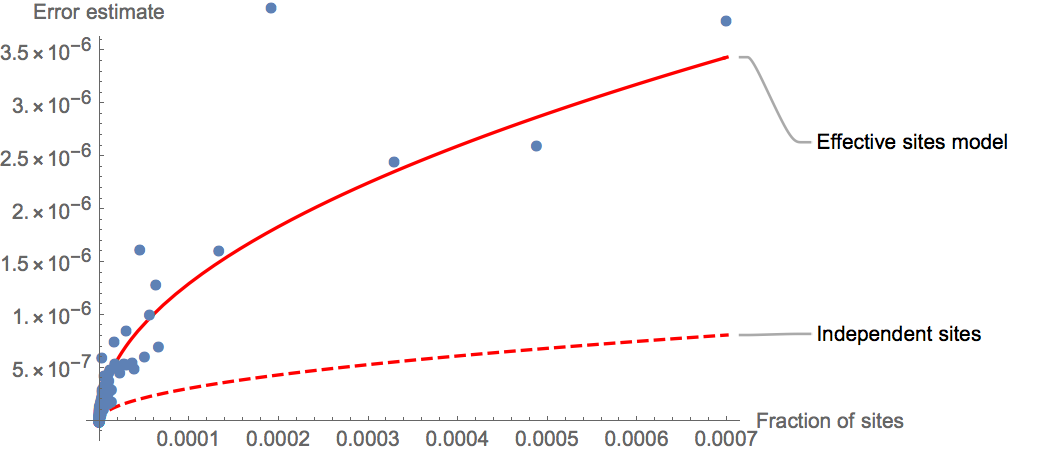
Under a true independent sites model without genetic linkage, the errors should follow a simple Poisson error model (dashed line), which predicts a square-root relationship between the error and the frequency of an observation. Specifically, the relationship between errors \(\Delta x\) and frequency \(x\) should be:
where \(N\) is the number of callable sites.
As can be seen, the true error estimates are much higher than under the independent sites assumption, which naturally reflects genetic linkage. We can then fit a simple “Effective sites” model to the observed errors (solid line), by simply reducing the total number of callable sites by a factor \(\alpha\). Specifically, we fit the function
inferring the parameter \(\alpha\) by a simple least-square fit. In this example we estimate \(\alpha=0.055\), which means that the inferred effective number of sites is about 18 times smaller than the true number of sites.
When using rarecoal mcmc, you can use the option --effectiveSitesReduction=0.055 to input this factor and have the likelihood being decreased by that factor, which automatically will increase the posterior confidence intervals.